Credit Assignment in Reinforcement Learning

The problem of credit assignment is a long-lasting issue in reinforcement learning. In short, it’s about which action is actually “caused” the reward in the future. Here I am looking at two papers that address this problem.

• Synthetic Returns for Long-Term Credit Assignment
• Counterfactual Credit Assignment

Synthetic Returns for Long-Term Credit Assignment (24th Feb 2021)

1-step TD error approach to learning suffers with delayed rewards with long periods or when between the action and reward there are uncontrollable events that contribute.

Their proposed method (optimizing synthetic returns, explanation will come later) combined with the IMPALA agent is able to solve the skiing game in Atari, which is difficult because of the delayed reward, 25 times faster than the state of the art of the time.

State-associative learning. The goal is to learn associations between pairs of states such that the state that was visitied prior to the other one is predictive of the reward and the future state (I think a better word here would be future timestep). This enables the algorithm to construct a synthetic return that connects the reward to the previous state by skipping timesteps.

Door-key example. If you have a door that you need to open to receive reward, you first need to pick up the key. So the credit of the reward shold be assigned to the state (transition) before (pickiping up the key), otherwise with one-step TD error we are going to obtain no reward signal for the key pickup transition and the value function approximator has a hard time of figuring this out, a lot of samples are needed.

Equation 1., the reward prediction loss. This is a bit weird to me, since the gating function $g(s_t)$ gates (softly) the sum over the outputs of $c(s_k)$ for T previous states and we have the baseline subtracted. So the prediction of the reward is in fact the sum of the state predictions. What is also a bit weird is that this is the internal agent state and not the actual environment observation (since partially observable). That should mean that the state $s_{t-1}$ of the previous states contains a summary of the history, should be predictive of the reward at $s_t$. There is no notion of causality here, i.e. which transition actually caused the reward. In the end, the augmented reward that they use is ${\hat{r}}_t=\alpha c(s_t)+\beta r_t$

Apparently there is a JAX implementation of this, yuppee!

Alright, a bit later after the equation they explain why they are summing over $c(s_k)$, the motivation is that the reward prediction is cast as a regression problem with weights, so each of the past states has a certain “weight” that is associated with their prediction, meaning how relevant is their prediction. It must have something to do with the architecture of the reward predictor, it’s still somewhat ad-hoc to me since there are no regression weights in the sum.

Synthetic return. This is what they call $c(s_k)$.

Further, they assume that the contribution of past states to a future state reward is sparse, that’s why the gating mechanism is introduced before the sum. I think it probably didn’t work without the gating mechanism, because there is no causal connection here between past action and reward, this might be a problem worth exploring.

Notice that the baseline in Eq. 1 depends on $s_t$ and is subtracted, the argument here is that $b(s_t)$ can still overtake the prediction of the reward in spite of the previous states, but I don’t see any way how it is encouraged to do so actually. Apparently, re-using $c(\cdot )$ didn’t work as well as using a separate function for this.

The $\alpha$ and $\beta$ hyperparameters are there because of the trade-off between this useful inductive bias that 1-step TD error has (that temporal recency is a good indicator for reward attribution) and this synthetic return. Are there any nice properties of this in the tabular case actually?.

Experiments. I am pretty much skipping this section in interest of time, long story short - the algorithm is very good in cases of long delayed rewards. The only thing that is peculiar to me that the objective for the synthetic returns is modified.

Summary/Discussion Do I don’t get it here why are they calling it a synthetic return instead of a synthetic reward, which it is. They mention that they cannot offer convergence guarantees because of the use of multiplicative gates and because of the use of an additive regression model they cannot offer guarantees for optimal credit assignment :), but the cool things is that they propose SA variants that overcome this in the appendix. Another problem is that this method has high variance across seeds for some reason.

BONUS: Appendix. In the current formulation the reward contributions of the summation might be double counted, so there is no reward conservation. The section 6.4 limitation of additive regression I am not getting exactly, now suddenly we have the function $c(\cdot ,\cdot )$, I need to read this more thoroughly.

Counterfactual Credit Assignment

Key idea: condition value functions on future events by learning to extract relevant information from a trajectory.

Let’s jump to the method section right away, I’m just gonna say it straight, I don’t like the notation style… Who uses $\mathcal{X}$ for state space in RL, observation is $E_t$ and $S_t$ the score function , come on :D … Note that, the score function is basically ${\mathrm{\nabla }}_{\theta }\log {\pi }_{\theta }(a|x)$. Equation 1 indicates REINFORCE, so the point here is that it’s a Monte-Carlo estimate! So the only thing that we need to do is to be able to simulate trajectories (a lot of them though!). Another feature here is the value function baseline in this formulation (I believe that the original REINFORCE didn’t have value function baseline?). A key feature of REINFORCE is that the likelihood of an action increases proportionally to the return from time-step t, not the whole trajectory. Second feature is that subtracting $V(X_t)$ does not bias the estimator and typically reduces the variance, the baseline is normally assumed not to depend on future observations this is kind of the motivator of this paper.

Weber et al (2019) showed that including variables that are causally dependent on the action leads to a biased estimator.

The REINFORCE estimator actually updates only the single action that was taken in the trajectory, but there is work from Sutton (2000) (would be interest to read this) that shows that we can derive a policy gradient estimator that actually updates all of the actions simultaneously. It is basically summing across all of the timesteps of the trajectory discounted and summing over all of the actions where we weight the score function with $Q(X_t,a)$. I don’t understand this sentence after eq. 2: “… this is in contrast with score function estimates above which depend on the return, a function of the entire trajectory” actually, this is true yes, the REINFORCE gradient weights all of the timesteps by difference between $G_t-V(X_t)$.

Hindisght reasoning vs. luck. Imagine a team game where the agent is a weak player and it plays with a strong player in a team. The team wins, but what should the agent learn from this positive reward signal, since all of the actions that it has taken have not contributed to victory.

Buesing et al. (2019) show that hindsight information is helpful in understanding the trajectory, pretty frequently. This work is connected to the work of Buesign et al. with the difference that this work focuses on model-free and the other is model-based.

Here's a thought I think that this future-conditioned baseline is predicting returns that are not influenced by the policy, whatever the policy does or in fact, maybe this can be formulated as predicting the worst-case return?

Future-conditional PG. The point here is that the baseline can be conditioned on future information, but there needs to be a importance correction term because otherwise future-conditioned policy gradients would be biased. How bad is this bias?

Theorem 1. FC-PG Assumption in the main text is that the (policy) - (action density conditioned on statistic and state) ratio needs to be finite, i.e. 0 cannot be in the denominator. In fact, this improtance ratio is used for correction in fron of $V(X_t,{\varphi }_t)$, apparently there are no requirements to ${\varphi }_t$ with the correction term. The aforementioned assumption means that knowing the statistic ${\varphi }_t$ shouldn’t make the action taken by the policy completely unaffecting the future (hmmm… is this a big assumption actually?).

The FC-PG doesn’t necessarily have lower variance than classical PG, because of the importance weighting, the countermeasure to this is to study an estimator that makes the ratio equal to 1, meaning that the action is completely independent of the statistic ${\varphi }_t$, ie $p(a|X_t,{\varphi }_t)=\pi (a|X_t)$. And this is what leads us to CCA-PG, i.e. counterfactual gradient estimate.

Theorem 2. CCA-PG. Interesting theoretical result here is that the variance of CCA is at most the variance of the classical policy gradient and it has no bias, the only condition is that $A_t$ is independent of ${\varphi }_t$.

How do we estimate ${\varphi }_t$? This paper proposes three methods, the interesting result is Theorem 3.. We consider a general variable $Y_t$ that is a function of the whole trajectory (known in hindsight) if we learn a generative model with latent variable ${ϵ}_t$ such that ${ϵ}_t\text{ind}{A}_t$, such that we compute by marginalizing out ${ϵ}_t$

$$p(Y_t|A_t,X_t)=\int p({ϵ}_t|X_t)p(Y_t|X_t,A_t,{ϵ}_t)d{ϵ}_t$$

Note, we are allowed to do so because of independence, but $Y_t$ is not assumed to be independent from the action. This probabilistic model induces the posterior $p({ϵ}_t|A_t,X_t,Y_t)$, if we sample ${\varphi }_t$ from this posterior, then it’s going to be conditionally independent of $A_t$ given $X_t$. This is a bit weird, since the posterior conditions on the action. But as it turns out, 1 sample is conditionally independent but a collection of samples wouldn’t be, i.e. a single sample form the posterior recovers conditional independence properties of the prior.

Corollary 1. I don’t understand this really, it’s basically taking the conditional expectation of $V(X_t,{ϵ}_t)$ with respect to the distribution $p({ϵ}_t|X_t,A_t,Y_t)$, and somehow this results in obtaining $V(X_t,A_t,Y_t)$, the formula is correct, but I don’t get the intuition because normally it’s only $V(X_t)$ how the value is defined, Corrolary 2 is a similar story.

Learning CCA with Generative Models. Figures, we need a generative model, so the first idea that comes to mind for modelling the posterior are Variational Autoencoders.

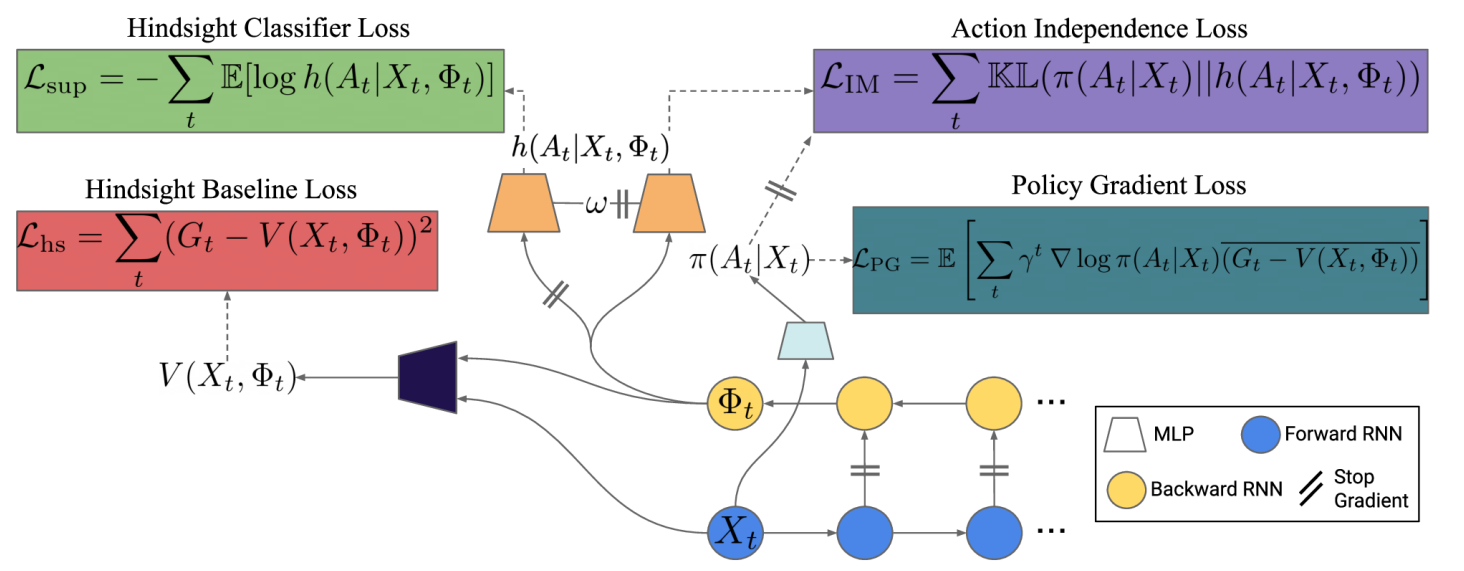
Model-free approach to learning CCA. Method related to domain-adversarial training techniques (whatever that is). Two objectives guide the learning signal: (1) $V(X_t,{\varphi }_t)$ should be predictive of the outcome. (2) encourage ${\varphi }_t$ to be conditionally independent of the outcome, this is done by simply minimizing the KL divergence between action classifiers $p(A_t|X_t)$ and $p(A_t|X_t,{\varphi }_t)$, obviously this is only 0 if $A_t\text{ind}{\varphi }_t$.

Practical implementation. They use an RNN so that the algorithm is applicable to POMDPs. A hindsight network is used for predicting ${\varphi }_t$ and a hindsight preidctor that outputs a distribution over $A_t$ and is used to enforce the independence condition.

Causality

Connections to causality. Assume that the MDP is generated by a structural causal model and that the return $G_t$ is calculated as a deterministic function $f(X_t,A_t)$, the exogenous variables of the SCM (i.e. those without causal ancestors represent the things that $A_t$ cannot influence but affect the return). The agent does not know the exact values of the exogenous variables $\mathcal{E}$ but tries to implicitly estimate them (by minimizing the KL that I talked about earlier). This is relatively clear, since we are maximizing the information contained about the outcome in ${\varphi }_t$ while minimizing the information about the action $A_t$.

Notion of counterfactuals in SCMs. In simple terms, you need to keep in mind that counterfactual distributions are different from conditionals. Why? First of all, because of mutilating the DAG, the incoming arrows of the variables that we intervene on are deleted. But more importantly, we are asking ourselves the question: “What would have happened, if I acted differently, under the same conditions”. This means that the exogenous variables are fixed, in other words, we are also conditioning on the exogenous variables. Now, the authors here give a neat definition of conterfactuals with some fancy terminology:

• Abduction: infer the exogenous variables $ϵ$
• Intervention: fix values of certain variables, here we are fixing $A_t$.I was a bit confused by this at first, but later on they write $p(\tau |\text{observe}(\tau ),\text{do}(A_t^{\prime }=a_t^{\prime })$, which makes sense since we are keeping all the conditions, except the intervened ones, the same, it’s just a bit funky to read.
• Prediction: self-explanatory, just infer the counterfactual outcome (values of variables)

Theorem 4. counterfactual distribution identifiability. Now, the golden question is how do we identify this counterfactual distribution, since we are not given the exogenous variables explicitly. It turns out that given the assumptions of faithfulness (classic) and conditional independence of ${\varphi }_t$, the counterfactual distribution is identifiable given samples of $(X_t,{\varphi }_t,A_t)$. Moreover, if we compute the expected return given this distribution, this is equal to $Q(X_t,A_t,{\varphi }_t)$. Commentary: As a turn of events, we don’t know how good ${\hat{\varphi }}_t$ really is, this can break down if we have bad estimates - another example where approximation is slipped into the theory to make it work in real :).